Chapter 6: Statistics: Normal Distribution
Objective
Here you will learn how to use the Empirical Rule to estimate the probability of an event.
If the price per pound of USDA Choice Beef is normally distributed with a mean of $4.85/lb and a standard deviation of $0.35/lb, what is the estimated probability that a randomly chosen sample (from a randomly chosen market) will be between $5.20 and $5.55 per pound?
Watch This: Empirical Rule
Guidance
This reading on the Empirical Rule is an extension of the previous reading “Understanding the Normal Distribution.” In the prior reading, the goal was to develop an intuition of the interaction between decreased probability and increased distance from the mean. In this reading, we will practice applying the Empirical Rule to estimate the specific probability of occurrence of a sample based on the range of the sample, measured in standard deviations.
The graphic below is a representation of the Empirical Rule:
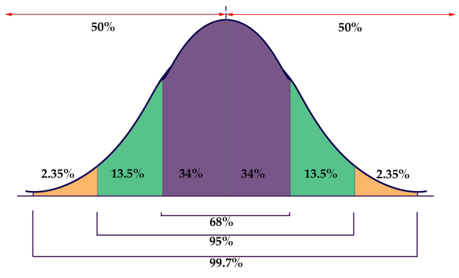
The graphic is a rather concise summary of the vital statistics of a Normal Distribution. Note how the graph resembles a bell? Now you know why the normal distribution is also called a “ bell curve.”
- 50% of the data is above, and 50% below, the mean of the data
- Approximately 68% of the data occurs within 1 SD of the mean
- Approximately 95% occurs within 2 SD’s of the mean
- Approximately 99.7% of the data occurs within 3 SDs of the mean
It is due to the probabilities associated with 1, 2, and 3 SDs that the Empirical Rule is also known as the 68−95−99.7 rule.
Example 1
If the diameter of a basketball is normally distributed, with a mean (µ) of 9″, and a standard deviation (σ) of 0.5″, what is the probability that a randomly chosen basketball will have a diameter between 9.5″ and 10.5″?
Solution
Since the σ = 0.5″ and the µ = 9″, we are evaluating the probability that a randomly chosen ball will have a diameter between 1 and 3 standard deviations above the mean. The graphic below shows the portion of the normal distribution included between 1 and 3 SDs:
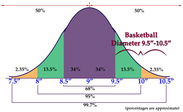
The percentage of the data spanning the 2nd and 3rd SDs is 13.5% + 2.35% = 15.85%
The probability that a randomly chosen basketball will have a diameter between 9.5 and 10.5 inches is 15.85%.
Example 2
If the depth of the snow in my yard is normally distributed, with µ = 2.5″ and σ = .25″, what is the probability that a randomly chosen location will have a snow depth between 2.25 and 2.75 inches?
Solution
2.25 inches is µ − 1σ, and 2.75 inches is µ + 1σ, so the area encompassed approximately represents 34% + 34% = 68%.
The probability that a randomly chosen location will have a depth between 2.25 and 2.75 inches is 68%.
Example 3
If the height of women in the United States is normally distributed with µ = 5′ 8″ and σ = 1.5″, what is the probability that a randomly chosen woman in the United States is shorter than 5′ 5″?
Solution
This one is slightly different, since we aren’t looking for the probability of a limited range of values. We want to evaluate the probability of a value occurring anywhere below 5′ 5″. Since the domain of a normal distribution is infinite, we can’t actually state the probability of the portion of the distribution on “that end” because it has no “end”! What we need to do is add up the probabilities that we do know and subtract them from 100% to get the remainder.
Here is that normal distribution graphic again, with the height data inserted:
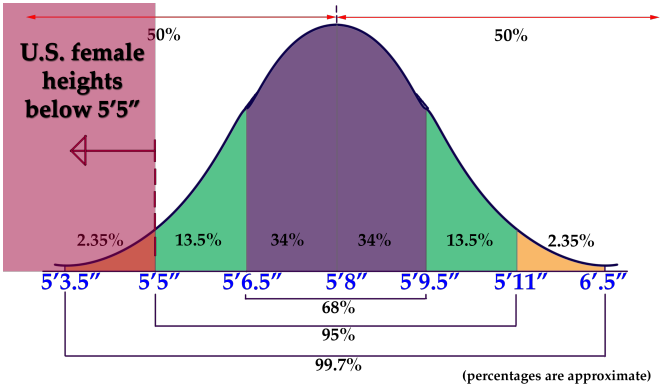
Recall that a normal distribution always has 50% of the data on each side of the mean. That indicates that 50% of US females are taller than 5′ 8″, and gives us a solid starting point to calculate from. There is another 34% between 5′ 6.5″ and 5′ 8″ and a final 13.5% between 5′ 5″ and 5′ 6.5″. Ultimately that totals: 50% + 34% + 13.5% = 97.5%. Since 97.5% of US females are 5′ 5″ or taller, that leaves 2.5% that are less than 5′ 5″ tall.
Intro Problem Revisited
If the price per pound of USDA Choice Beef is normally distributed with a mean of $4.85/lb and a standard deviation of $0.35/lb, what is the estimated probability that a randomly chosen sample (from a randomly chosen market) will be between $5.20 and $5.55 per pound?
$5.20 is µ + 1σ, and $5.55 is µ + 2σ, so the probability of a value occurring in that range is approximately 13.5%.
Vocabulary
Normal distribution: a common, but specific, distribution of data with a set of characteristics detailed in the lesson above.
Empirical Rule: a name for the way in which the normal distribution divides data by standard deviations: 68% within 1 SD, 95% within 2 SDs and 99.7 within 3 SDs of the mean
68-95-99.7 rule: another name for the Empirical Rule
Bell curve: the shape of a normal distribution
Guided Practice
- A normally distributed data set has µ = 10 and σ = 2.5, what is the probability of randomly selecting a value greater than 17.5 from the set?
- A normally distributed data set has µ = .05 and σ = .01, what is the probability of randomly choosing a value between .05 and .07 from the set?
- A normally distributed data set has µ = 514 and an unknown standard deviation, what is the probability that a randomly selected value will be less than 514?
Solutions
- If µ = 10 and σ = 2.5, then 17.5 = µ + 3σ. Since we are looking for all data above that point, we need to subtract the probability that a value will occur below that value from 100%: The probability that a value will be less than 10 is 50%, since 10 is the mean. There is another 34% between 10 and 12.5, another 13.5% between 12.5 and 15, and a final 2.35% between 15 and 17.5. 100% −50% −34% −13.5% −2.35% = 0.15% probability of a value greater than 17.5
- 0.05 is the mean, and 0.07 is 2 standard deviations above the mean, so the probability of a value in that range is 34% + 13.5% = 47.5%
- 514 is the mean, so the probability of a value less than that is 50%.
Attributions
This chapter contains material taken from Math in Society (on OpenTextBookStore) by David Lippman, and is used under a CC Attribution-Share Alike 3.0 United States (CC BY-SA 3.0 US) license.
This chapter contains material taken from of Math for the Liberal Arts (on Lumen Learning) by Lumen Learning, and is used under a CC BY: Attribution license.
